Der Asisstent meinte, dass das mit der Sakllierung und Orientierung nicht so tragisch sei, bzw. das wir uns das in der Übungsstunde noch einmal zusammen genauer ansehen werden. Er wollte aber, dass ich das mit den Farben versuche zu ändern..
Ich habe einmal deinen Vorschlag versucht, Problem ist dabei, dass wohl gewisse Werte dann keinen Sinn machen, bzw. nicht richtig interpretiert werden. Der Fehler in der cmd lautet:
Ich denke ich lasse mal den Rest des Codes da, sonst wird es wohl schwer hier eine Lösung zu finden.
Code: Alles auswählen
from numpy import *
from numpy.linalg import eig, norm
from scipy.special import hermite, gamma
from matplotlib.pyplot import *
def arnoldi(A, v0, k):
r"""Arnoldi algorithm to compute the Krylov approximation :math:`H` of a matrix :math:`A`.
:param A: The matrix :math:`A` of shape :math:`N \times N` to approximate.
:param v0: The initial vector :math:`v_0` of length :math:`N`.
:param k: The number :math:`k` of Krylov steps performed.
:return: A tuple :math:`(V, H)` where :math:`V` is the large matrix of shape
:math:`N \times (k+1)` containing the orthogonal vectors and :math:`H` is the
small matrix of shape :math:`k \times k` containing the Krylov approximation
of :math:`A`.
"""
r, c = A.shape
V = zeros((r, k+1), dtype=complexfloating)
H = zeros((k+1, k), dtype=complexfloating)
V[:,0] = v0.reshape(-1) / norm(v0)
for i in range(1, k+1):
vi = dot(A, V[:,i-1])
for j in range(i):
H[j,i-1] = dot(conjugate(V[:,j]), vi)
vi -= H[j,i-1] * V[:,j]
H[i,i-1] = norm(vi)
V[:,i] = vi / H[i,i-1]
return V, H[:-1,:]
def Part3():
# Teil 3: Unteraufgaben g), h), i)
# Harmonischer Osillator
v = lambda x, y: 0.5*(x**2 + y**2)
# Henon-Heiles
a = 2.0
b = 0.4
v = lambda x, y: 0.5*a*(x**2 + y**2) + b*(x**2*y - y**3/3.0)
N = 32
x, h = linspace(-3, 3, N, retstep=True)
X,Y = meshgrid(x,x)
x = X.reshape(-1)
y = Y.reshape(-1)
# Just K for later use
K = 6
# Unteraufgabe g)
# Laplace Part
D = zeros((N*N, N*N), dtype=floating)
for r in range(0, N):
for c in range(0, N):
# X direction stencil
if c == 0:
# Forward
D[N*r+c, N*r+c] += 1.0
D[N*r+c, N*r+(c+1)] += -2.0
D[N*r+c, N*r+(c+2)] += 1.0
elif c == N-1:
# Backward
D[N*r+c, N*r+(c-2)] += 1.0
D[N*r+c, N*r+(c-1)] += -2.0
D[N*r+c, N*r+c] += 1.0
else:
# Central
D[N*r+c, N*r+(c-1)] += 1.0
D[N*r+c, N*r+c] += -2.0
D[N*r+c, N*r+(c+1)] += 1.0
# Y direction stencil
if r == 0:
# Forward
D[N*r+c, N*r+c] += 1.0
D[N*r+c, N*(r+1)+c] += -2.0
D[N*r+c, N*(r+2)+c] += 1.0
elif r == N-1:
# Backward
D[N*r+c, N*(r-2)+c] += 1.0
D[N*r+c, N*(r-1)+c] += -2.0
D[N*r+c, N*r+c] += 1.0
else:
# Central
D[N*r+c, N*(r-1)+c] += 1.0
D[N*r+c, N*r+c] += -2.0
D[N*r+c, N*(r+1)+c] += 1.0
D /= h**2
# Potential Part
V = diag(v(x,y))
# Hamiltonian
H = -0.5*D + V
figure()
matshow(H[:50,:50])
colorbar()
savefig("discrete_hamiltonian.pdf")
# Unteraufgabe h)
ew, ev = eig(H)
# Sort the eigenvalues
I = argsort(ew)
ew = ew[I]
Psi = ev[:,I]
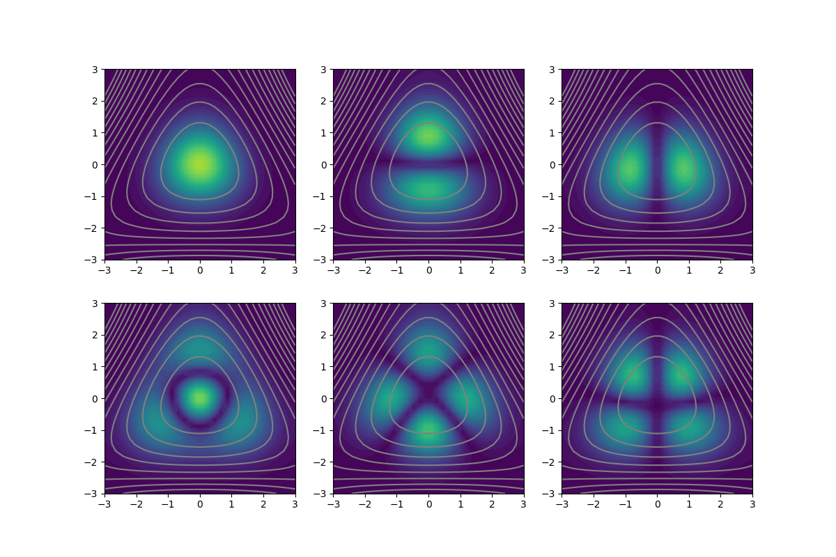
fig = figure(figsize=(12,8))
for k in range(K):
# Plot first K eigenstates
psik = Psi[:,k].reshape((N,N))
fig.add_subplot(2, 3, k+1)
ax = fig.gca()
ax.set_aspect('equal')
ax.contour(X, Y, v(X,Y), colors="gray", levels=linspace(0, 20, 15))
ax.contourf(X, Y, abs(psik), levels=linspace(0, 0.15, 40))
#ax.grid(True)
fig.savefig("henon_eigenfunctions.pdf")
# Unteraufgabe i)
# Startvektor fuer Arnoldi
v0 = ones(N*N)/N
VK, HK = arnoldi(H, v0, 220)
ewk, evk = eig(HK)
I = argsort(ewk)
ewk = ewk[I]
evk = evk[:,I]
Psik = dot(VK[:,:-1], evk)
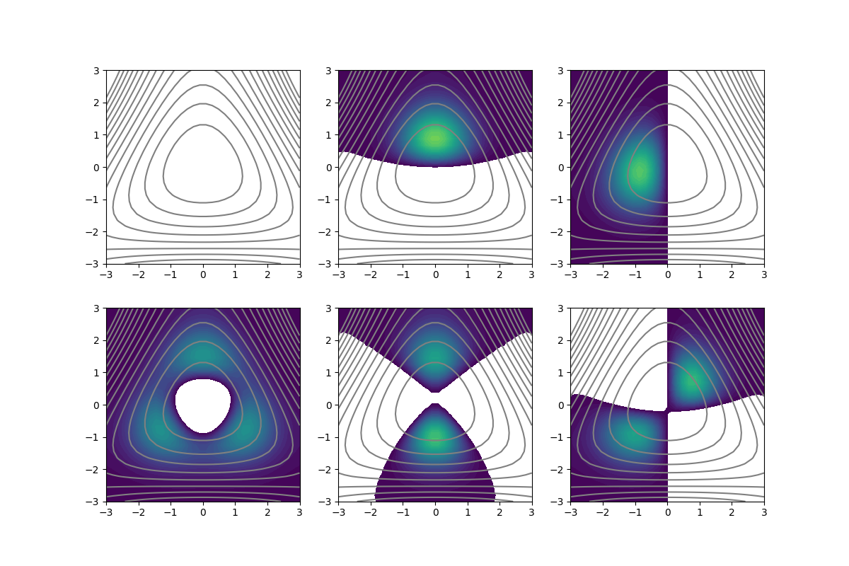
fig = figure(figsize=(12,8))
vc = 0
for k in range(0, 2*K):
# Skip some numerical artefacts
if abs(ewk[k]) < 1.0:
continue
else:
vc += 1
if vc > K:
break
# Plot first K eigenstates
        psik = Psik[:,k].reshape((N,N))

        fig.add_subplot(2, 3, vc)
        ax = fig.gca()
        ax.set_aspect('equal')

        ax.contour(X, Y, v(X,Y), colors="gray", levels=linspace(0, 20, 15))
        ax.contourf(X, Y, abs(psik), levels=linspace(0, 0.15, 40))
#ax.grid(True)
fig.savefig("henon_eigenfunctions_arnoldi.png")
if __name__ == "__main__":
Part3()